
B-K Tree is a data structure for efficient similarity search. It provides logarithmic insertion and search operations, if the distance metric follows triangle inequality, e.g. hamming (for bit arrays), Levenshtein (edit distance for strings), Euclidean distances (say between word embeddigns).
Idea
The idea is a very neat recursive process.
build([nodes...]). Given a list of nodes, choose any one to be the root. It then buckets the remaining nodes based on their distances to the root. For each distance, and its corresponding nodes, choose any one to be the child of root and apply the samebuild()process recursively.insert(root, node). It starts from the root, obtain the distance between root and node, and locates the substree, whose root ischild. If the subtree (child) is empty, node is inserted as child of root. Otherwise, recursively applyinsert(child, node).search(root, target, tolerance).toleranceis the max distance difference accepted betweentargetand any node. Whentolerance=0, the search is an exact match. The key idea is a constraint scope tranversal. The process maintains an open set of candidates (usually implemented as queue or stack). It starts from the root, obtain the distancedbetween root and node, and add all children whose distances are in the range[d - tolerance, d + tolerance]to the candidates (important!). It pops the candidates and recursively add their children in the same way. During the tree tranversal, we note the nodes whose distance to target is within tolerance.
Complexity
We use hamming distance as an example, to articulate the complexity is logarithmic in a probabilistic way.
Hamming distance essentially measures the number of different bits between two bit arrays.
Suppose a given target is at a very deep leaf node. The path from root to this target has a distance sequence of (d1, d2, d3, ... dL), where L is the depth (aka "level") of final hop.
No matter what is the dx, there is 1/ 2^m probabiliy that distance between our target and the particular child has a distance of dx, where m is size of each element (aka number of bits). The joint probability that a path tranverses distances in exact order of (d1, d2, d3, ... dL), is simply (1/ 2^m) ^ (L-1). This is the probability that one random target follows a path of depth-L. For n nodes in the tree, the expectation of # of nodes that follow a depth-L or more path is (1/ 2^m) ^ (L-1) * n.
We solve (1/ 2^m) ^ (L-1) * n >= 1 for L, and gets L <= 1/m log(n) + 1. That means, in order to have at least one node that has depth L, L needs to be smaller than a logarithmic function of n, which is the problem size.
The proof is not rigorous but to give some intuition of the BK tree's core design. The key observation is that, when L increases, the chance that we can see a leaf node decays exponentially.
Once we show that the tree is of logarithmic depth, and the search range at each layer is a bounded constant irrelevant of n, we can conclude that both the insert() and search() are of logarithmic complexity.
Correctness
The key for BK tree's efficiency roots from the constraint scope search by selection children whose distances are in the range [d - tolerance, d + tolerance] .
Let's see why the nodes outside this range can be safely excluded. Consider a node c of current root p, which has distance greater than d+tolerance. We denote target node as t. Then we have below relations:
distance(c, p) > d+tolerance(via search constraints)distance(t, p) = d(via BK Tree definition, akabuild()algorithm)distance(c, t) + distance(t, p) >= distance(c, p)(triangle inequality of distance)
Rearranging the last one, we can get distance(c, t) >= distance(c, p) - distance(t, p) = distance(c, p) - d > d + tolerance - d = tolerance.
Since distance(c, t) > tolerance, we can safely exclude the node and the subtree (all subtree nodes have the same distance as c, by the definition).
Experiments
We use pybktree in this experiment.
The dataset is a search query and keyword matching dataset.
- Query: total 692084 lines.
- Keyword: total 2735298 lines.
The distance is given by dist_levenshtein, which is a python only DP-implementation of Levenshtein distances.
Cost by size using exact match
We set tolerance to 0 for exact match.
By varying the number of query and keyword, we have the below results:
- query=10000, keyword=10000, build 3.3952s, match 3.7635s
- query=100000, keyword=100000, build 47.8441s, match 53.4976s
- query=692084, keyword=2735298, build 417.1134s, match 6349.2519s
The implementation works Ok on a single Macbook, at the size of 100K. When the problem size approaches millions level, it takes two hours to execute the matching phase.
Comments:
- Every node is represented as a Python dict
{}, which incurrs large overhead. We will show some statistics later that the majority nodes has a breadth of 0, aka no children. We can change the implementation to save memory. - dist_levenshtein is bounded by the multiplication of sizes of string 1 and string 2. It is a constant in theory, but the factor could be large. A more primitive C implementation could accelerate this.
- We can divide the both query set and keyword set into multiple chunks and do the build+match on all the chunks. The process can be parallelized for speed-up. The total computation CPU time, however, could be larger. For example, suppose we divide the chunks with 100K chunk size, and re-use the results from second line of the experiments. The total CPU time is 27 x 7 x (48s + 54s) = 19,278, which is larger than 6349 seconds on the third line.
Cost by tolerance
We fix query=10000 and keyword=10000 in this experiment, and change the tolerance.
- tolerance=0, build 3.3386s, match 4.5119s, avg candidates 4.5668
- tolerance=1, build 3.4580s, match 46.5436s, avg candidates 86.1188
- tolerance=2, build 3.3154s, match 284.9257s, avg candidates 429
- tolerance=3, build 3.4160s, match 529.4454s
When the tolerance increases, the constraint search scope increases by 2x the tolerance. This is exponential in depth L. BK Tree only works well when the tolerance is small. In our experiment, even with 3-character edit distane tolerance, matching 10,000 keywords already takes minutes.
The last number in above list shows the average candidates for one search. The denominator is 10,000. We can see that less than 5% of the queries were searched with a tolerance=3. The search space pruning is still effective.
Tree statistics
In order to better understand the tree's shape, we take the statistics for each node:
- Breadth: how many child does this tree have.
- Depth: the number of hops along the root-to-node path.
We define two types of order of insert() , random and sequential. Sequential is a string sort of the input texts.
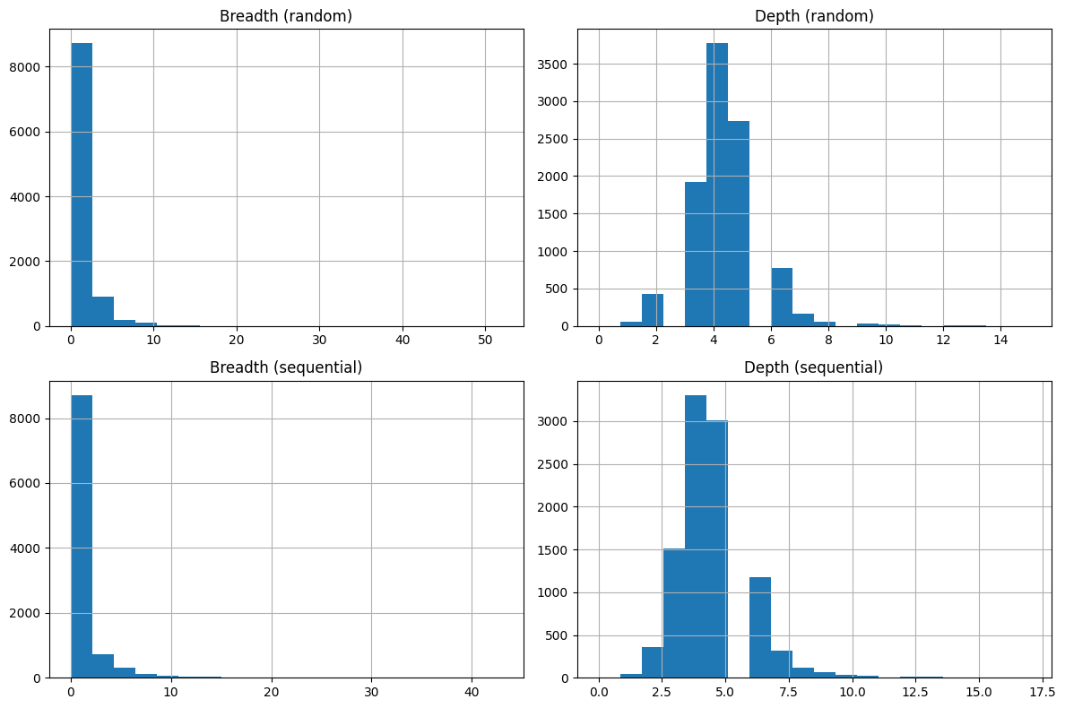
We can see that:
- Insert order does not matter much for the distribution of breadth and depth.
- 60% of the nodes do not have children (breadth=0).
- 90% quantile of breadth is 3.
- median of depth is 4.
- 99% quantile of depth is 8. --- this is a strong evidence that BK Tree's depth is low.
We can further comprehend the experiment results in the last chapter using the statistics here. Suppose a depth of 8, and a tolerance tot. The number of all candidates for a given search() task is (2 * tot) ^ 8. This number is irrelevant of problem size, but increases dramatically with respect to the tolerance level.
About the author
Just run the code, or yourself.
Comments
Join the discussionHello everyone,
If you're having issues withdrawing, swapping, or selling ETHM (EthereumMeta), LUSD, Thoreum V3, 4WMM, BTCBR, or any other tokens, we can help.
Many projects experience migration errors, liquidity loss, or contract issues that lock funds. Whether it's meme coins, DeFi tokens, or abandoned projects, our team specializes in recovering inaccessible assets.
For secure assistance, contact us at: email📩rexasfinance99@gmail.com